Paper Reading - Attention Is All You Need

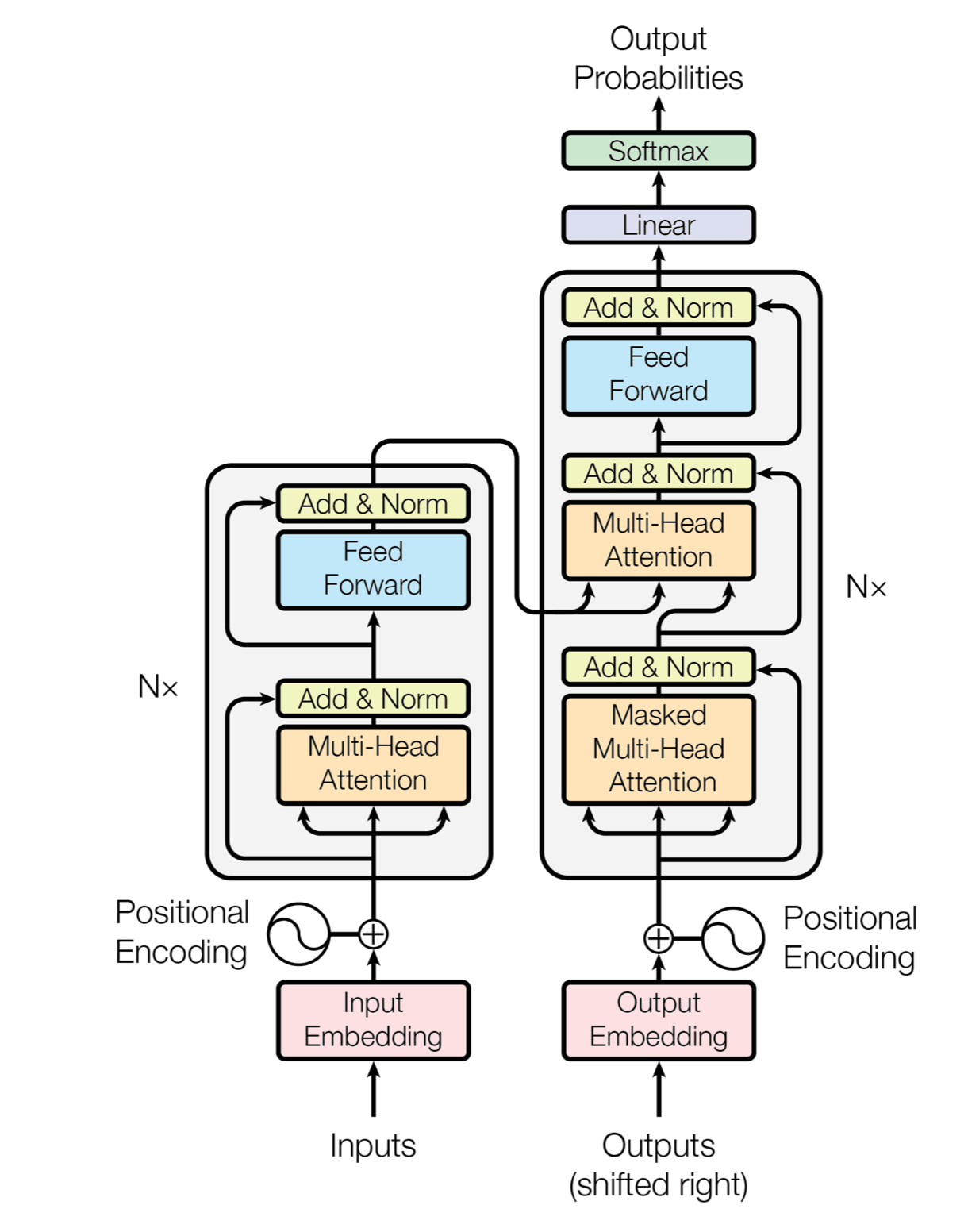
Google的这篇论文提出了一个只使用Attention机制的神经翻译模型，该模型依旧采用编码器-解码器（Encoder-Decoder）架构，但未使用RNN和CNN。文章的主要目的是在减少计算量和提高并行效率的同时不损害最终的实验结果，创新之处在于提出了两个新的Attention机制，分别叫做 Scaled Dot-Product Attention 和 Multi-Head Attention.

整体框架

整体框架

• 输入：一个句子 \(z = (z_1, …, z_n)\)，它是原始句子 \(x = (x_1, …, x_n)\) 的 Embedding，其中 \(n\) 是句子长度。
• 输出：翻译好的句子 \((y_1, …, y_m)\)

Encoder

• 输入 \(z \in R^{n \times d_{model}}\)
• 输出大小不变
• Positional Encoding
• 6个Block
  • Multi-Head Self-Attention
  • Position-wise Feed Forward
  • Residual connection
    • LayerNorm(x + Sublayer(x))
    • 引入了残差，尽可能保留原始输入x的信息
  • \(d_{model} = 512\)

Decoder

• Positional Encoding
• 6个Block
  • Multi-Head Self Attention (with mask)
    • 采用 0-1mask 消除右侧单词对当前单词 attention 的影响
  • Multi-Head Self Attention (with encoder)
    • 使用Encoder的输出作为一部分输入
  • Position-wise Feed Forward
  • Residual connection

Multi-Head Self Attention

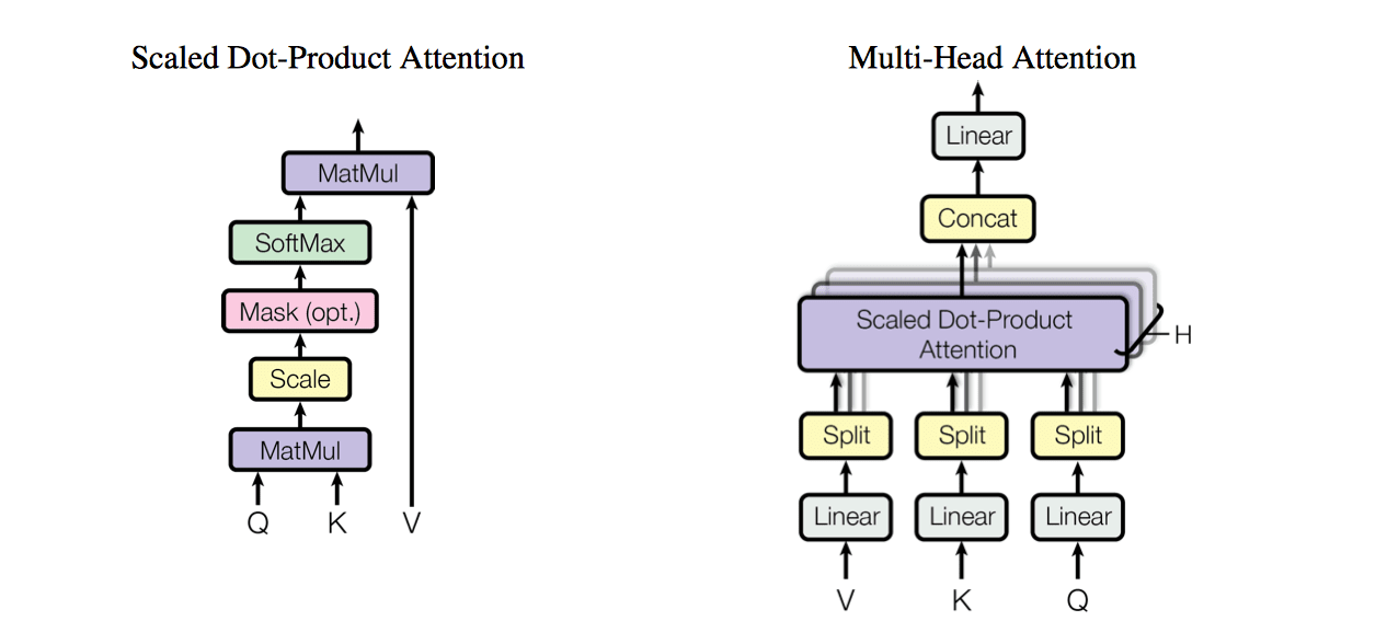
Multi-Head Attention

输入 \(Q \in R^{n \times d_{model}}\)、\(K \in R^{n \times d_{model}}\)、\(V \in R^{n \times d_{model}}\)，分别代表query、key-value pair。这里的 key, value, 和 query 需要解释一下，这里把 attention 抽象为对 value (\(V\)) 的每个 token 进行加权，而加权的 weight就是 attention weight，而 attention weight 就是根据 query 和 key 计算得到，其意义为：为了用 value 求出 query 的结果, 根据 query 和 key 来决定注意力应该放在 value 的哪部分。以前的 attention 是用 LSTM 做 encoder，也就是用它来生成 key 和 value ，然后由 decoder 来生成 query。具体到 Bahdanau 的论文 Neural machine translation by jointly learning to align and translate，key 和 value 是一样的，都是文中的 \(h\)，而 query 是文中的 \(s\)。而在这篇论文中：

• 在encoder块中，key, value, query 同为encoder_input（上一层的输出），因为是self-attention，可以理解为生成对这个句子的编码，可以全面获取输入序列中positions之间依赖关系。
• 在decoder块中，第一层Multi-Head Attention的输入都为decoder_input；第二层的 \(Q\) 为前一层的输出，\(K, V\) 为encoder的输出。可以理解为，比如刚翻译完主语，接下来想要找谓语，【找谓语】这个信息就是 query，然后 key 是源句子的编码，通过 query 和 key 计算出 attention weight （应该关注的谓语的位置），最后和 value （源句子编码）计算加权和。

然后把 \(Q, K, V\) 线性映射 \(h\) 次，分别映射到 \(d_k, d_k, d_v\) 维度，总的attention为每个映射的attention连接起来（这 \(h\) 个attention可以并行计算），即：

其中，投影的参数矩阵 \(W^Q_i \in R^{d_{model} \times d_k}\), \(W^K_i \in R^{d_{model} \times d_k}\), \(W^V_i \in R^{d_{model} \times d_v}\). 在论文中 \(h = 8\)，\(d_k = d_v = \frac{d_{model}}{h} = 64\)，所以这层的输出和输入大小相同。

这些线性映射使得模型可以从不同的子空间的不同位置中学习注意力！

Scaled Dot-Product Attention

上式中的attention正是Scaled Dot-Product Attention，它也接收 \(Q, K, V\) 三个参数，计算方法如下： \[ Attention(Q, K, V) = softmax(\frac{QK^T}{\sqrt{d_k}})V \] Dot-Product指的是 \(QK^T\)，scaled是指除以了 \(\sqrt{d_k}\) （因为假设两个 \(d_k\) 维向量每个分量都是一个相互独立的服从标准正态分布的随机变量，那么他们的点乘的方差就是 \(d_k\)，每一个分量除以 \(\sqrt{d_k}\) 可以让点乘的方差变成 1）。

总共有两种流行的attention计算方法：

• additive attention
  • 通过一个小型神经网络计算注意力
• dot-product attention
  • 上面的方法

其中第二种方法比第一种方法快很多，第一种方法在 \(d_k\) 较大时比第二种方法表现好，论文作者觉得可能是因为dot-product使梯度变得很大以至于失去作用，所以进行了scale。

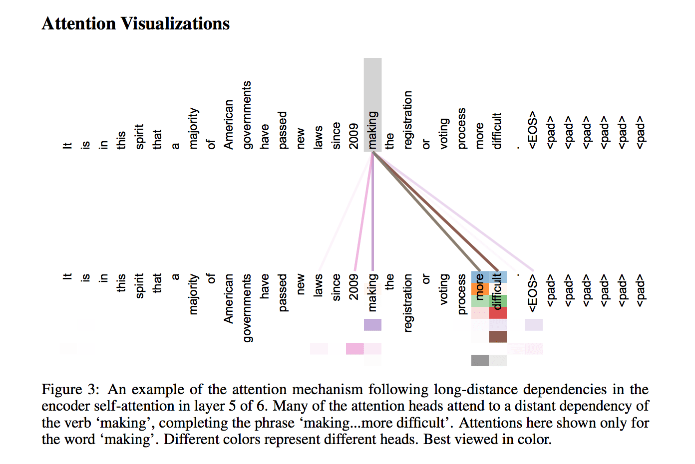
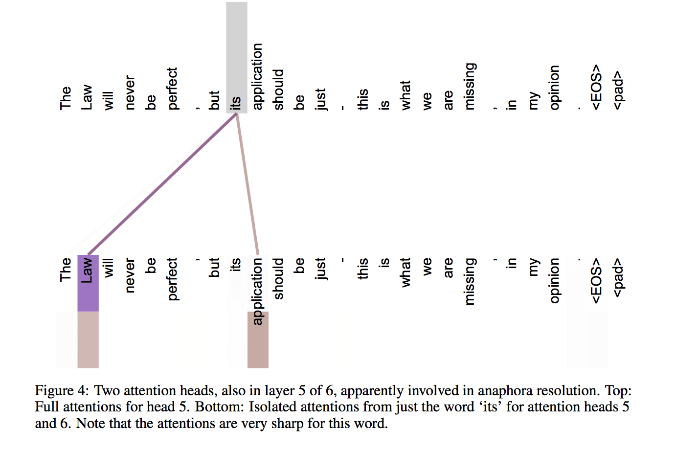
可视化 self-attention

Position-wise Feed-Forward Networks

\[ FFN(x) = \max(0, xW_1 + b_1)W_2 + b_2 \]

这是一个 MLP （多层）网络，上层的输出中，每个 \(d_{model}\) 维向量 \(x\) 在此先由 \(xW_1+b_1\) 变为 \(d_{ff}\) 维的 \(x'\)，再经过 \(\max(0, x')W_2+b_2\) 回归 \(d_{model}\) 维。之后再是一个 residual connection。输出大小和输入大小一样，都 \(\in R^{n \times d_{model}}\).

Positional Encoding

因为这个网络没有 recurrence（因为decoder在训练时给ground truth做为输入，这样生成不同位置的词是可以并行的）和 convolution，为了表示词在序列中的位置信息，要用一种特殊的位置编码。

本篇论文中使用 \(\sin\) 和 \(\cos\) 来编码： \[ \begin{array}{lcl} PE_{(pos, 2i)} & = & \sin(\frac{pos}{10000^{2i/d_{model}}})\\ PE_{(pos, 2i+1)} & = & \cos(\frac{pos}{10000^{2i/d_{model}}}) \end{array} \] 其中，\(pos\) 代表位置，\(i\) 代表维度（\([0, d_{model}-1]\)）。

这样做的目的是因为正弦和余弦函数具有周期性，对于固定长度偏差 \(k\)（类似于周期），\(pos+k\) 位置的 PE 可以表示成关于 \(pos\) 位置 PE 的一个线性变换（\(\sin(pos + k) =\sin(pos)\cos(k)+\sin(k)\cos(pos)\)），这样可以方便模型学习词与词之间的一个相对位置关系。

另一种解释，来自 WarBean ：

每两个维度构成一个二维的单位向量，总共有 \(d_{model} / 2\) 组。每一组单位向量会随着 \(pos\) 的增大而旋转，但是旋转周期不同，按照论文里面的设置，最小的旋转周期是 \(2\pi\)，最大的旋转周期是 \(10000 \times 2\pi\)。至于为什么说相邻 \(k\) 步的 position embedding 可以用一个线性变换对应上，是因为上述每组单位向量的旋转操作可以用表示为乘以一个 2 x 2 的旋转矩阵。

特点

1. 训练阶段完全可并行（因为decoder在训练时给ground truth做为输入，这样生成不同位置的词是可以并行的，而encoder一次处理一整个句子）

2. 解决 long dependency 的问题

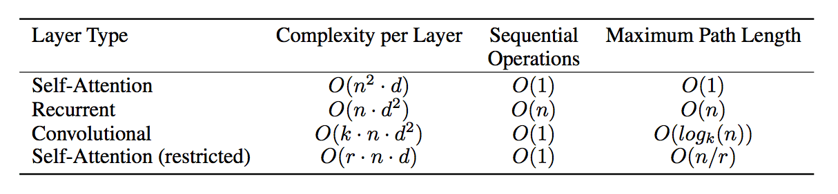
   传统的用RNN建模语言的时序特征，前面的单词信息都依次feed到后面一个单词，这种信息的堆叠感觉有点浪费，而且反而把信息糅杂在一起不好区分，虽然decoder阶段对每个单词对应的encoder输出位置做attention，但每个encoder输出已经夹杂了前面单词的信息。同时前面单词信息往后传，走的路径比较长，也就是long dependency的问题，虽然LSTM/GRU这种结构能一定程度上解决，但是毕竟不能完全去掉 long dependency。而conv在处理dependency问题时，利用卷积的感受野receptive field，通过堆叠卷积层来扩大每个encoder输出位置所覆盖单词的范围，每个单词走的路径大致是logk(n)步，缩短了dependency的长度。而这篇论文的做法是直接用encoder或者decoder的层与层之间直接用attention，句子中的单词dependency长度最多只有1，减少了信息传输路径。而且这种attention的方式直接可以挖掘句子内部单词与单词的语义组合关系，将它作为一个语义整体，使得翻译时更好地利用单词组合甚至是短语的信息，更好地decode出语义匹配的目标语言单词（转自谭旭）

开源代码分析

代码来自：https://github.com/jadore801120/attention-is-all-you-need-pytorch

使用 PyTorch 框架

Encoder

class Encoder(nn.Module):
    ''' A encoder model with self attention mechanism. '''

    def __init__(self, n_src_vocab, n_max_seq, n_layers=6,
                 n_head=8, d_k=64, d_v=64,
        		 d_word_vec=512, d_model=512, 
                 d_inner_hid=1024, dropout=0.1):
        # .....

    def forward(self, src_seq, src_pos):
        # Word embedding look up
        enc_input = self.src_word_emb(src_seq)

        # Position Encoding addition
        enc_input += self.position_enc(src_pos)
        enc_outputs, enc_slf_attns = [], []

        enc_output = enc_input
        enc_slf_attn_mask = 
        		get_attn_padding_mask(src_seq, src_seq)
        # 对每一层计算 encoder output 和 self-attention
        for enc_layer in self.layer_stack:
            enc_output, enc_slf_attn = enc_layer(
                enc_output, slf_attn_mask=enc_slf_attn_mask)
            # 把每层的输出添加到总输出列表
            enc_outputs += [enc_output]
            enc_slf_attns += [enc_slf_attn]

        return enc_outputs, enc_slf_attns

Positional Encoding

def position_encoding_init(n_position, d_pos_vec):
    ''' Init the sinusoid position encoding table '''
	# 对每个位置进行编码，位置0为全0，其他位置按照相应公式计算
    position_enc = np.array([
        [pos / np.power(10000, 2*i/d_pos_vec) 
        	for i in range(d_pos_vec)]
        if pos != 0 else np.zeros(d_pos_vec) 
        	for pos in range(n_position)])
	# dim 2i
    position_enc[1:, 0::2] = np.sin(position_enc[1:, 0::2]) 
    # dim 2i+1
    position_enc[1:, 1::2] = np.cos(position_enc[1:, 1::2]) 
    return torch.from_numpy(position_enc)

Scaled Dot-Product Attention

class ScaledDotProductAttention(nn.Module):
    ''' Scaled Dot-Product Attention '''

    def __init__(self, d_model, attn_dropout=0.1):
        super(ScaledDotProductAttention, self).__init__()
        self.temper = np.power(d_model, 0.5)
        self.dropout = nn.Dropout(attn_dropout)
        self.softmax = BottleSoftmax()

    def forward(self, q, k, v, attn_mask=None):
        attn = torch.bmm(q, k.transpose(1, 2)) / self.temper
        ...
        attn = self.softmax(attn)
        attn = self.dropout(attn)
        output = torch.bmm(attn, v)

        return output, attn

从中可见，self-attention 指 softmax 操作之后的部分，层输出是 \(attention \times V\)。

Encoder layer

class EncoderLayer(nn.Module):
    ''' Compose with two layers '''

    def __init__(self, d_model, d_inner_hid, n_head, d_k, d_v,
                 dropout=0.1):
        super(EncoderLayer, self).__init__()
        self.slf_attn = MultiHeadAttention(
            n_head, d_model, d_k, d_v, dropout=dropout)
        self.pos_ffn = PositionwiseFeedForward(d_model, 
                                              d_inner_hid, 
                                              dropout=dropout)

    def forward(self, enc_input, slf_attn_mask=None):
        # Q, K, V 都是 enc_input
        enc_output, enc_slf_attn = self.slf_attn(
            enc_input, enc_input, enc_input,
            attn_mask=slf_attn_mask)
        enc_output = self.pos_ffn(enc_output)
        return enc_output, enc_slf_attn

可见，传给 MultiHeadAttention 的\(Q, K, V\) 都是 enc_input。

Decoder Layer

class DecoderLayer(nn.Module):
    ''' Compose with three layers '''

    def __init__(self, d_model, d_inner_hid, n_head, d_k, d_v, dropout=0.1):
        # ....

    def forward(self, dec_input, enc_output, 
                slf_attn_mask=None, dec_enc_attn_mask=None):
        # 第一个attention层接收的 Q, K, V 都是 dec_input
        dec_output, dec_slf_attn = self.slf_attn(
            dec_input, dec_input, dec_input, 
            attn_mask=slf_attn_mask)
        # 第二个attention层接收的 Q 是 dec_output，
        # K 和 V 是 enc_output
        dec_output, dec_enc_attn = self.enc_attn(
            dec_output, enc_output, enc_output, 
            attn_mask=dec_enc_attn_mask)
        dec_output = self.pos_ffn(dec_output)

        return dec_output, dec_slf_attn, dec_enc_attn

Transformer

class Transformer(nn.Module):
    ''' 完整的 transformer '''

    def __init__(
            self, n_src_vocab, n_tgt_vocab, n_max_seq,
        	n_layers=6, n_head=8, d_word_vec=512, d_model=512,
        	d_inner_hid=1024, d_k=64, d_v=64, dropout=0.1,
        	proj_share_weight=True, embs_share_weight=True):

        super(Transformer, self).__init__()
        # 初始化 encoder
        self.encoder = Encoder(
            n_src_vocab, n_max_seq, n_layers=n_layers,
            n_head=n_head, d_word_vec=d_word_vec, 
            d_model=d_model, d_inner_hid=d_inner_hid,
            dropout=dropout)
        # 初始化 decoder
        self.decoder = Decoder(
            n_tgt_vocab, n_max_seq, n_layers=n_layers,
            n_head=n_head, d_word_vec=d_word_vec, 
            d_model=d_model, d_inner_hid=d_inner_hid,
            dropout=dropout)
      	# ....

    def forward(self, src, tgt):
        src_seq, src_pos = src
        tgt_seq, tgt_pos = tgt

        tgt_seq = tgt_seq[:, :-1]
        tgt_pos = tgt_pos[:, :-1]
		# 编码
        enc_outputs, enc_slf_attns = self.encoder(src_seq,
                                                  src_pos)
        # 解码
        dec_outputs, dec_slf_attns, dec_enc_attns =
        	self.decoder( tgt_seq, tgt_pos, src_seq,
                         enc_outputs)
        dec_output = dec_outputs[-1]

        seq_logit = self.tgt_word_proj(dec_output)

        return seq_logit.view(-1, seq_logit.size(2))